Chapter 11

Discrete co(sin) transform at a glance. Main reasons of why is it predominantly used in lossy (video) image compression systems.
Let us recapitulate the main steps of processing a video frame as it is being encoded using a H.265/HEVC system (Fig. 1). At the first step, termed conventionally “block division”, the frame is divided into blocks called CUs (Coding Units). The second step involves predicting the image inside each block using spatial (Intra) or temporal (Inter) prediction. When temporal prediction is being performed, a CU block can be divided into sub-blocks called PUs (Prediction Units), each of which can have its own motion vector. The predicted sample values are then subtracted from the sample values of the image being coded. As a result, a two-dimensional (2D) difference signal, or Residual signal, is formed for each CU. At the third step, the 2D array of Residual signal samples is divided into so-called TUs (Transform Units) that undergo a 2D discrete cosine Fourier transform (with the exception of the 4×4-sized TUs containing intra-predicted intensity samples, for which a discrete sine Fourier transform is used).
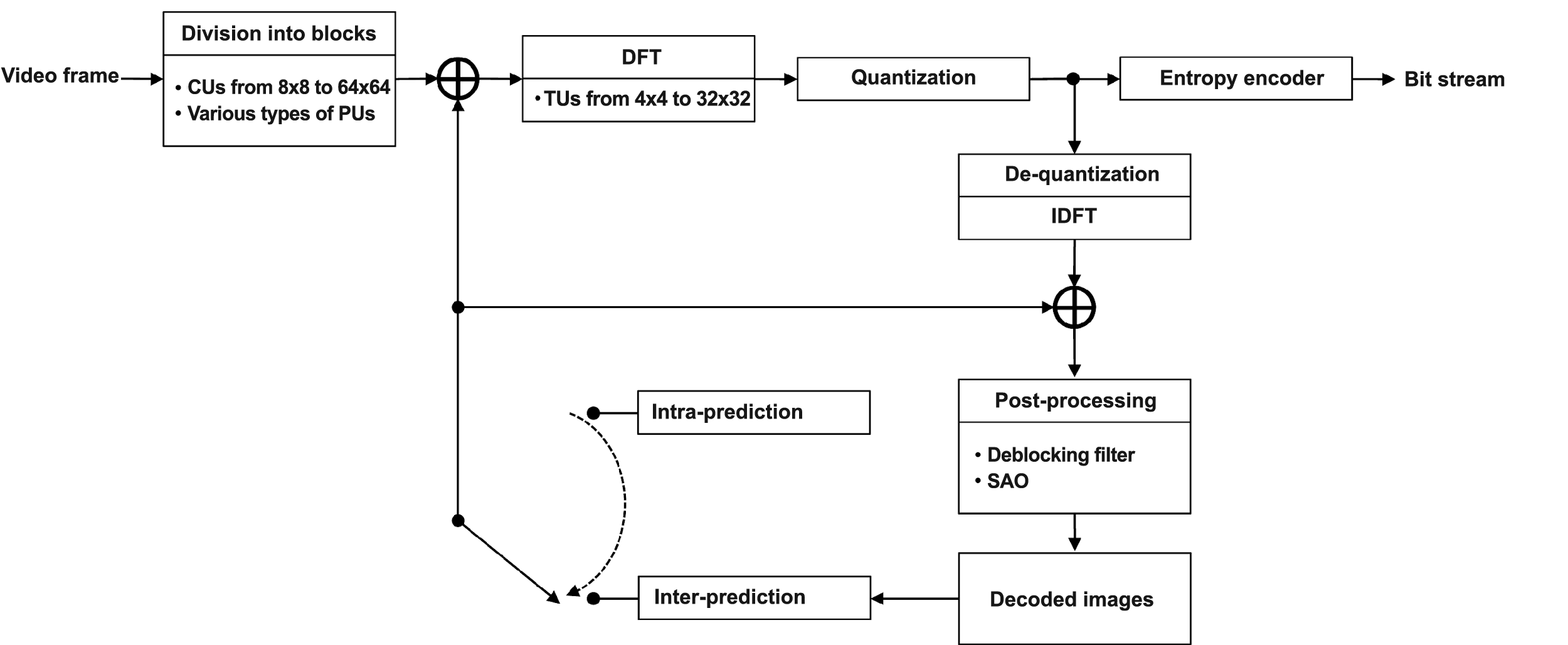
Figure 1. Main stages of video frame encoding in a H.265/HEVC system
Then the resulting spectral Fourier coefficients of the Residual signal are quantized by level. At the final step, the data about all operations performed at each of the four stages are sent to the input of an entropy encoder. This data can be used later to restore the encoded image. The entropy encoder performs additional lossless compression on the incoming data using Context Adaptive Binary Arithmetic Coding (CABAC) algorithms.
This article aims to explain what happens with the video image at the third compression step. Why is a discrete (co)sine transform used there? Why is the discrete cosine transform (DCT) used predominantly in lossy (video) image compression systems? (Lossy compression systems are ones where the compression stage introduces distortion, and a decoded image is always different from the original as a result.) These are the questions we will try to answer.
Why is the DCT used predominantly in lossy (video) image compression systems? To answer this question, we need to invoke some results from the theory of random processes that were initially obtained by Hotelling and published in 1933. Hotelling proposed a method of representing time-discrete random processes as a set of uncorrelated random coefficients. During the 1940s, Karhunen and Loève published papers proposing a similar representation for time-continuous random processes. Both the discrete and the continuous transforms are now referred to as the Karhunen-Loève transform, or eigenvector decomposition, in most of the digital signal processing literature. Let us summarize these results here for the specific case of a 2D discrete random process (image).
The Karhunen-Loève transform is given by
\begin{array}{l}Y( u,v) =\sum ^{N-1}_{j=0} \ \ \sum ^{M-1}_{k=0} \ \ X( j,k) \ \ W( j,k,u,v),\\\end{array}
where $\displaystyle X(j,k) $ denotes the discrete samples of the digital image, and the transform kernel $\displaystyle W(j,k,u,v) $
\begin{array}{l} \lambda ( u,v) W( j,k,u,v) \ =\ \sum ^{N-1}_{i=0} \ \sum ^{M-1}_{l=0} \ K( j,k,i,l) W( i,l,u,v),\\\end{array}
where $\displaystyle K(j,k,i,l) $ is the covariance function of the digital image, and $\displaystyle \lambda(u,v)$ is constant for fixed values of $\displaystyle u,v$ is generally considered that the covariance function $\displaystyle K(j,k,i,l) $ of a digital image is separable—that is, it can be expressed as a product
\begin{array}{l}K(j,k,i,l) =K_{C}(j,k)K_{R}(i,l),\\\end{array}
where $\displaystyle K_{C}(j,k) $ is the vertical image covariance, j and k are pixel row indices, $\displaystyle K_{R}( i,l)$ is the horizontal image covariance, and i and l are pixel column indices. If the covariance is separable, the Karhunen-Loève transform kernel is also separable, and the transformation can be applied first for columns and then for rows (or vice versa). In this case, the Karhunen-Loève transform kernel can be expressed as
\begin{array}{l}W\ ( j,k,u,v) \ =\ \ W_{C}( j,k) W_{R}( u,v),\\\end{array}
and each term in the product satisfies its own equation:
\begin{array}{l}\lambda _{R}( v) W_{R}( i,v) =\sum ^{M-1}_{l=0} \ K_{R}( i,l) W_{R}( l,v),\\\end{array}
and
\begin{array}{l}\lambda _{C}( u) W_{C}( j,u) =\sum ^{N-1}_{k=0} \ K_{R}( j,k) W_{R}( k,u).\\\end{array}
Thus, the Karhunen-Loève transform makes it possible to represent a digital image as a set of uncorrelated random variables. But how does this help? What is so remarkable about this representation? The Transform and Data Compression Handbook edited by K.R. Rao and P.C. Yip. (Boca Raton, CRC Press LLC, 2001) answers this in the most comprehensible way. In the chapter on the Karhunen-Loève transform, the authors consider the following experiment. They propose dividing the image into non-overlapping blocks as shown in Figure 2 (taken from the book).
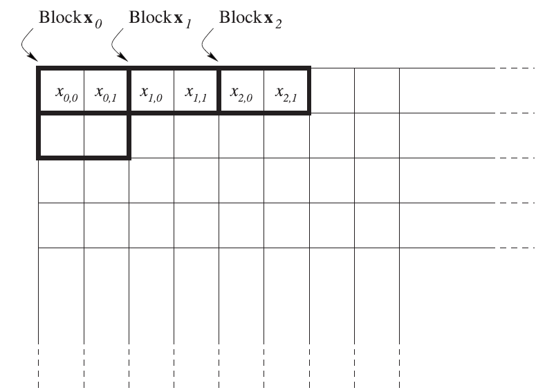
Figure 2. Main stages of video frame encoding in a H.265/HEVC system
The two set of blocks completely defines the image being processed. As a result, the image is represented as a set of 2D vectors, $\displaystyle \overrightarrow{x_{i}} =(x_{i0},x_{i1})$ The scatter plot for the entire vector set $\displaystyle \overrightarrow{x_{i}} $ where the point positions are defined by the coordinates of the vectors $\displaystyle \overrightarrow{x_{i}} $ is shown in Figure 3 (taken from the book).
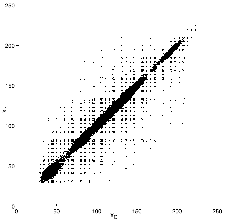
Figure 3. Scatter plot for the vectors $\displaystyle \overrightarrow{x_{i}} $
It can be seen from the plot in Figure 3 that the values of adjacent pixels are strongly correlated (a 45-degree straight line is clearly visible). Figure 4 (taken from the book) shows histograms of $\displaystyle x_{i0} $ and $\displaystyle x_{i1} $ values.
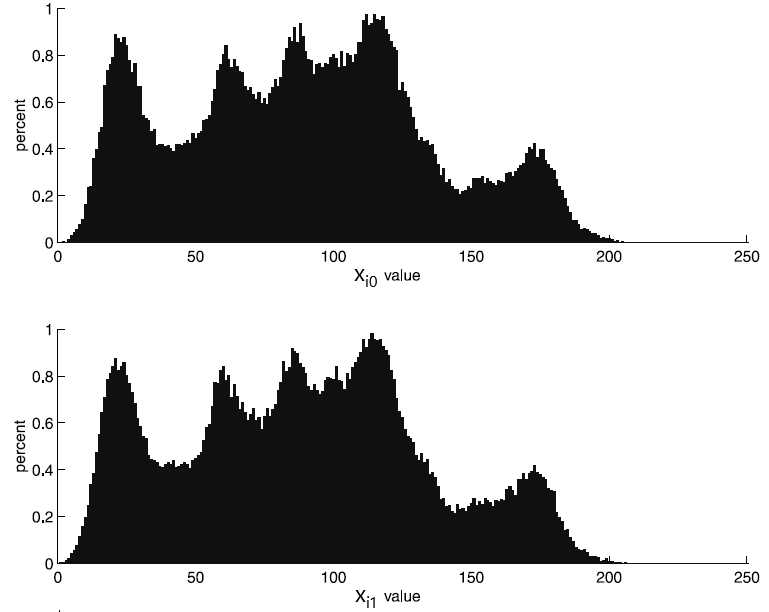
Figure 4. Histograms of $\displaystyle \overrightarrow{x_{i0}} $ and $\displaystyle \overrightarrow{x_{i1}} $ pixel values
The Karhunen-Loève transform turns vectors $\displaystyle \overrightarrow{x_{i}} $ into vectors $\displaystyle \overrightarrow{y_{i}} $ with coordinates $\displaystyle ({y_{i0}},{y_{i1}}) $. The scatter plot for the vectors $\displaystyle \overrightarrow{y_{i}} $ shown in Figure 5 (taken from the book) exhibits no correlation between the coordinates of the vectors $\displaystyle \overrightarrow{y_{i}} $.

Figure 5. Scatter plot after a Karhunen-Loève transform
Figure 6 (taken from the book) shows histograms of $\displaystyle y_{i0} $ and $\displaystyle y_{i1} $ values.
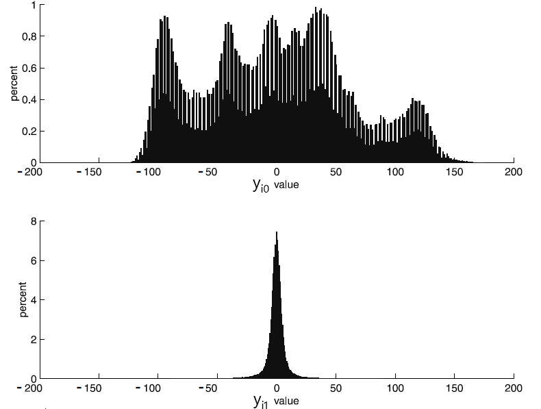
Figure 6. Histograms of coordinate values for the vectors $\displaystyle \overrightarrow{y_{i}} $ .
As evident from the histogram, the dynamic range of the $\displaystyle {y_{i0}} $ values is virtually the same as the initial one (i.e. the range of values $\displaystyle {x_{i0}} $). However, the second component, $\displaystyle {y_{i1}} $ now has a dramatically different dynamic range. The histogram for this coordinate has only a fraction of the $\displaystyle {x_{i1}} $ histogram width. Clearly, the smaller the dynamic range of a given quantity, the fewer bits will be needed to represent this quantity digitally. Thus, even in a case as simple as transforming 2D vectors (which amounts to rotating the vectors by 45 degrees), the Karhunen-Loève transform compresses the image.
In the more general case where the $\displaystyle \overrightarrow{x_{i}} $ vectors have a greater length (as mentioned above, the general assumption used in image processing is that the 2D Karhunen-Loève transform is separable and can be performed successively in the horizontal and vertical directions), transforming them into vectors $\displaystyle \overrightarrow{y_{i}} $ with uncorrelated coordinates provides a higher compression ratio. Moreover, the coordinates of the $\displaystyle \overrightarrow{y_{i}} $ vectors turn out to be more robust to quantization. That is, if we quantize the coefficients of the Karhunen-Loève decomposition and then de-quantize them and perform a reverse transform, the error introduced at the quantization step will be a minimum (in the RMS sense) over all possible linear transforms. Discarding some number of final coefficients (i.e. the final coordinates of the $\displaystyle \overrightarrow{y_{i}} $ vectors) also gives the minimum RMS error. Therefore, the Karhunen-Loève transform provides the most compact placement of the $\displaystyle \overrightarrow{y_{i}} $ vectors in the first coordinates for the greatest amount of information contained in the $\displaystyle \overrightarrow{x_{i}} $ vectors. Of course, all of this makes the Karhunen-Loève transform virtually ideal for use in digital data compression systems, including image compression systems.
The Karhunen-Loève transform has one—but significant—disadvantage. The kernel of this transform is defined by the statistical nature of the data being processed and requires the above equations to be solved for each set of vectors $\displaystyle \overrightarrow{x_{i}} $. Analytical solutions for these equations are only known for some special cases. A numerical solution, while possible, is so computationally intensive that using the Karhunen-Loève for video image processing becomes virtually impractical.
One special case of random processes, for which an analytical solution of the Karhunen-Loève transform kernel equations is known, is that of type I Markov processes. The correlation function for such processes has an exponential form when their values have a normal (Gaussian) distribution. For a discrete one-dimensional random process, the correlation function $\displaystyle K(i,j) $ has the form
\begin{array}{l}K( i,j) \ = σ^{2} ρ ^{|i-j|},\\\end{array}
where $\displaystyle 0\leqslant ρ \leqslant 1$ It has been shown in the paper Relation between the Karhunen Loeve and cosine transforms (RJ.Clarke, B.Tech., M.Sc, C.Eng., Mem.I.E.E.E., M.I.E.E. IEEPROC, Vol. 128, Pt. F, No. 6, NOVEMBER 1981) that for $\displaystyle ρ → 1$, the solution obtained for a Markov process coincides with the Type II discrete cosine Fourier transform, or DCT-II (as is commonly known, eight types of this transform exist in total). On the other hand, numerous studies of statistical properties of digital images have shown that the horizontal $\displaystyle K_{R}(i,j) $ and vertical $\displaystyle K_{C}(i,j) $ correlation functions of images are exponential in form. The values of $\displaystyle ρ$ for both are close to 1 (ranging from 0.95 to 0.98). This means that for most images, DCT-II is a very good approximation to the Karhune-Loève transform, and the horizontal and vertical transform kernels have an identical form:
\begin{array}{l}W(i,k)=\begin{cases} \frac{1}{\sqrt{N}} & i=0,\ 0\leq k\leqslant N-1\\ \sqrt{\frac{2}{N}}\cos\left(\frac{i\pi ( 2k+1)}{2N}\right) & 0< i\leqslant N-1,\ 0\leqslant k\leqslant N-1 \end{cases}\\\end{array}
Let us return to the first question that was asked in the beginning of this article.
Why is a discrete (co)sine transform used at the third step? The reason for using DCT is clear: this transform is a good approximation to the Karhunen-Loève transform for most images, including those obtained by inter-prediction, i.e. for the residual signal. But where did the sine transform come from?
At the very beginning of the HEVC standard development, a research group from Singapore (Document: JCTVC-B024) showed that the correlation properties of the residual signal obtained by intra-prediction differ significantly from those of regular images and the residual signal obtained by inter-prediction. This is easy to understand: indeed, the residual signal samples located closest to the reference samples used for intra-prediction clearly have the smallest variance. The further the residual signal samples from the reference ones, the greater the variance. The researchers from Singapore proposed an analytical expression for the correlation function of the residual signal for horizontal and vertical intra-prediction. They also showed that the kernel of the Karhunen-Loève transform in these cases is the function
\begin{array}{l}W( i,j) =\frac{2}{\sqrt{2N+1}}\sin\frac{\pi ( 2i+1)( j+1)}{2N+1} ,\ 0\leq i,j\leq N-1\\\end{array}
that coincides with the kernel of the discrete sine Fourier transform.
April 9, 2021
Read more:
Chapter 1. Video encoding in simple terms
Chapter 2. Inter-frame prediction (Inter) in HEVC
Chapter 3. Spatial (Intra) prediction in HEVC
Chapter 4. Motion compensation in HEVC
Chapter 5. Post-processing in HEVC
Chapter 6. Context-adaptive binary arithmetic coding. Part 1
Chapter 7. Context-adaptive binary arithmetic coding. Part 2
Chapter 8. Context-adaptive binary arithmetic coding. Part 3
Chapter 9. Context-adaptive binary arithmetic coding. Part 4
Chapter 10. Context-adaptive binary arithmetic coding. Part 5
About the author:
Oleg Ponomarev, 17 years in video encoding and signal digital processing, expert in Statistical Radiophysics, Radio waves propagation. Assistant Professor, PhD at Tomsk State University, Radiophysics department. Head of Elecard Research Lab.