CHAPTER 3

Possible ways of eliminating temporal or spatial redundancy in video images. Block-by-block basis of image processing in HEVC. The procedure of spatial prediction: four major steps. Algorithms of calculation of the pixel values inside the block being coded.
Video coding systems implementing the HEVC standard are categorized as so-called hybrid block-based codecs. “Block-based” means here that each video frame is divided during the coding process into blocks to which the compression algorithms are then applied. So what does “hybrid” mean? To a large extent, the compression of video data during coding is achieved by eliminating redundant information from the video image sequence. Obviously, the images in the video frames that are adjacent in time are highly likely to appear similar to one another. To eliminate temporal redundancy, the previously coded frames are searched for the most similar image to each block to be coded in the current frame. Once found, this image is used as an estimate (prediction) for the video frame area being coded. The prediction is subtracted from the pixel values of the current block. In the case of a “good” prediction, the difference (residual) signal contains significantly less information than the original image, which provides efficient compression. However, this is just one way of eliminating redundancy. HEVC offers another option where the pixel values from the same video frame as the current block are used for prediction. This kind of prediction is called spatial or intra-frame prediction (Intra). Thus, what the term “hybrid” refers to is the use of the two possible ways of eliminating temporal or spatial redundancy in video images at the same time. It should also be noted that intra-prediction efficiency is what determines in large measure the efficiency of the coding system as a whole. Let us now consider in more detail the main ideas underlying the methods and algorithms of intra-prediction provided by the HEVC standard.
As already noted, image processing in a HEVC system is performed on a block-by-block basis. The process of dividing the video frame into blocks is adaptive – that is, tailored to the nature of the image. As a first step, the image is divided left to right and top to bottom into identical square blocks called LCUs (from Largest Coding Unit). The LCU size is a parameter of the encoding system and is specified before the coding starts. This size can take the values of 8x8, 16x16, 32x32, or 64x64. Each LCU can be divided into 4 square sub-blocks called CU, each of which is also divisible into smaller units. Therefore, the LCU is the root of a quad tree. The minimum CU size, or the minimum quad tree depth, is also a parameter of the encoding system and can take the values of 8x8, 16x16, 32x32, or 64x64. Spatial intra-prediction is performed in HEVC for square-shaped blocks called PUs (from Prediction Unit). The PU has the same size as the CU, with two exceptions. Firstly, the PU size cannot exceed 32x32, therefore a 64x64 CU contains four 32x32 PUs. Secondly, the CUs at the lowest level of the quad tree that have the minimum allowed size can be further divided into four square PUs of half the size. As a result, the set of valid PU sizes in HEVC comprises the following values: 4x4, 8x8, 16x16, and 32x32. An example of dividing an image into CUs and PUs is shown in Figure 1. The thicker solid line marks the LCU boundaries, while the thin solid line delimits the CU sub-blocks. The dotted line represents the PU boundaries in cases where a CU contains four PUs. The figures inside the blocks show the order in which the PUs are accessed during coding.
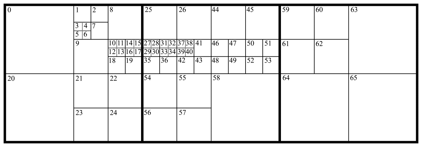
Figure 1.The LCU, CU, and PU boundaries (shown using thick solid, thin solid, and dotted lines respectively). The numbers inside the blocks show the block access order during coding
The spatial prediction of the pixel values inside the block to be coded is carried out in HEVC using the pixel values of the adjacent blocks. These are called reference pixels. Figure 2 shows where the reference pixels are located relative to the current block being coded. In this figure, the current block is marked with the letter C (with a size of 8x8 in this example). The letters A, B, D, E, and F denote the blocks that contain reference pixels. The pixel locations are shown in gray color. It is, however, far from always the case that all the reference pixels are available for use in prediction. Obviously, the pixels from blocks D, A, and B are not accessible to blocks 0, 1, 2, and 8 in Figure 1, because these blocks are located at the very top of the video frame. But this is not the only case when reference pixels are considered unavailable. According to the standard, only those reference pixels that are located in the already coded blocks are allowed to be used for prediction. This restriction makes it possible to decode each block after it has been encoded and then use the decoded pixels as reference. This ensures identical prediction results in the encoding and decoding systems. As an example, consider the availability of reference pixels for block 17 in Figure 1. When this block is being predicted, only the pixels from blocks A, D, and E are available for it as reference. The rest of the blocks surrounding block 17 have not yet been coded, given the specified access order, and hence cannot be used for prediction.
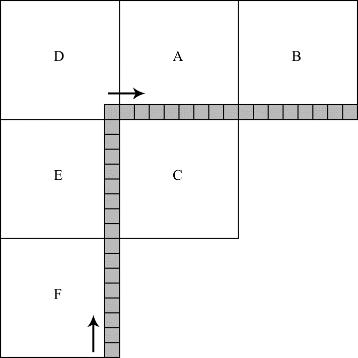
Figure 2. Reference pixel locations relative to the block being coded
In total, HEVC provides for 35 different variants of calculating the sample values in the area being coded based on reference pixel values when performing spatial prediction. These variants are called prediction modes. Each mode is identified by a unique number from 0 to 34.
The procedure of spatial prediction consists of four major steps, some of which are omitted for certain prediction modes and sizes of the block to be coded. The first step is to generate the values for the reference pixels that are not available, and it is always performed when there are unavailable samples. The process as such is very simple. All unavailable pixels are assigned the value of the first available sample. For instance, if blocks D, A, and B are not available (see Figure 2), then the reference pixels from all these blocks are assigned the value of the topmost reference sample from block E. If block B is not available, the entire row of samples in this block is assigned the value of the rightmost reference pixel from block A. The values for the vertical column of unavailable reference pixels are generated in a symmetrical fashion. Finally, if none of the blocks A, B, D, E, F is available, all the reference pixels are set at half the maximum possible value. If, for example, the samples in the video are represented by 8-bit numbers, then all the reference pixels are assigned a value of 127.
The second step of prediction is to filter the sequence of reference samples, accessing them first from bottom to top (i.e. from the bottommost sample in block F to the only sample in block D) and then from left to right (i.e. from the leftmost sample in block A to the rightmost sample in block B). The direction in which the samples are accessed during filtering is shown with arrows in Figure 2. The filter type is determined by the size of the block being coded. This step is omitted for certain prediction mode numbers and when predicting 4x4 blocks.
The third step involves the actual calculation of the pixel values inside the block being coded. Since the calculation algorithms vary significantly for different prediction modes, let us consider them in more detail. For that, we will need some basic math knowledge, specifically trigonometry.
Let us introduce the following notation. $\displaystyle N $ is the size of the block to be coded.$\displaystyle p(x,y) $ denotes the predicted values, where $\displaystyle x $ and $\displaystyle y $ are the coordinates of the predicted pixel inside the block to be coded. The upper left sample in the block has coordinates (0,0), while the lower left has coordinates $\displaystyle ( N-1,N-1) $. $\displaystyle t( x) $ is the sequence of the reference samples located above the block to be coded (blocks D, A, and B in Figure 2), where $\displaystyle x $ can take the values of –1, 0, 1, ... …$\displaystyle 2N-1 $. Finally, $\displaystyle l(y) $ is the column of reference samples located to the left of the block being coded, where the y coordinate can also take values in the range –1 to $\displaystyle ...2N-1 $. The notation just introduced is illustrated in Figure 3.
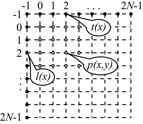
Figure 3. The notation used to describe intra-prediction modes
As already noted, each prediction mode is identified by a unique number. Let us proceed in ascending order.
Mode 0.
This is the so-called DC mode. In this mode, all $\displaystyle p(x,y) $samples are assigned the same value of $\displaystyle V_{DC} $ calculated as the arithmetic mean of the reference samples:
\begin{array}{l} V_{DC} =\left\lfloor \frac{1}{2N}\left(\sum _{x=0}^{N-1} t( x) +\sum _{y=0}^{N-1} l( x) +N\right)\right\rfloor \\\end{array}
where $\displaystyle\lfloor .\rfloor $ denotes the operation of taking the modulus of a number.
Mode 1.
Also called Planar mode. Each $\displaystyle p(x,y) $ value in this mode is obtained as the arithmetic mean of two numbers, $\displaystyle h( x,y) \ $ and $\displaystyle v( x,y) \ $. These numbers are calculated as a linear interpolation in the horizontal $\displaystyle ( h( x,y)) $ and vertical$\displaystyle ( v( x,y)) $ directions. The interpolation process is illustrated in Figure 4.
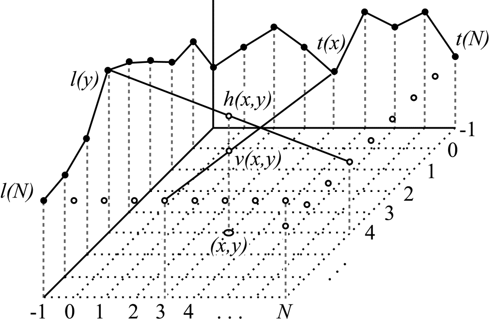
Figure 4. Interpolation in the horizontal and vertical directions
To calculate $\displaystyle h( x,y) \ $ the interpolation is carried out in the horizontal direction between the value of $\displaystyle l(y) $ and the value of $\displaystyle t(N) $ located $\displaystyle N+1 $ samples away from the latter. To calculate $\displaystyle v( x,y) \ $, the interpolation is performed between the value of $\displaystyle t(x) $ and the value of $\displaystyle l(N) $, also located $\displaystyle N+1 $ samples away in the vertical direction from the top horizontal row of reference pixels.
The calculations made in this mode can be described mathematically as follows:
\begin{array}{l} p( x,y) =\left\lfloor \frac{h( x,y) +v( x,y) +N}{2N}\right\rfloor \\\end{array}where
\begin{array}{l} h( x,y) =( N-1-x) l( y) +( x+1) t( N) \\\end{array}and
\begin{array}{l} v( x,y) =( N-1-y) t( x) +( y+1) l( N) \\\end{array}The remaining modes, numbered 2 to 34, are called angular modes. In these modes, the values of the reference samples in the specified direction are distributed inside the block to be coded. If the pixel $\displaystyle p(x,y) $ being predicted is located between reference samples, an interpolated value is used as the prediction. Two symmetrical groups can be identified in this set of modes. For modes 2 to 17, the reference values are distributed from left to right. For modes 18 to 34, they are distributed from top to bottom. The mapping between the mode number and the direction in which the reference samples are distributed is illustrated in Figure 5.
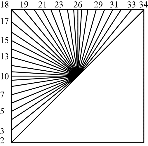
Figure 5. The numbers of angular prediction modes and the corresponding directions of reference sample distribution inside the block to be coded
Angular prediction modes 18 to 34.
For these modes, the angle $\displaystyle \varphi \ $ that is specified by the prediction mode number and determines the direction of sample distribution is taken from the vertical direction (see Figure 6). Modes 18 to 25 have negative values of $\displaystyle \varphi \ $, while modes 27 to 34 have positive values of this angle.
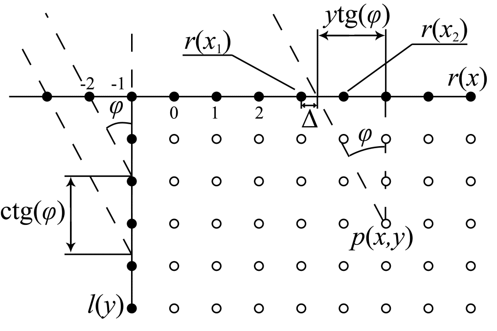
Figure 6. Angular prediction in the vertical direction
Let us consider how $\displaystyle p(x,y) $ is calculated, using Figure 6 as a reference. It is clear that the coordinate of the projection of the point $\displaystyle( x,y) $ onto the horizontal axis containing the reference samples (denoted as $\displaystyle r( x) $ in Figure 6, but more on that later) in the direction specified by the angle $\displaystyle \varphi \ $ can be expressed as:
\begin{array}{l} \ x\prime =x+y\tan( \varphi ) \\\end{array}When $\displaystyle x\prime $ coincides with the coordinate of a reference sample, the value of $\displaystyle r( \ x\prime ) $ is assigned to $\displaystyle p(x,y) $. This always happens when the projected coordinate $\displaystyle x\prime $ is an integer. In case of a non-integer $\displaystyle x\prime $ , $\displaystyle p(x,y) $ is calculated as a linear interpolation between the values of the reference samples $\displaystyle r( x_{1}) $ and $\displaystyle r( x_{2}) $ located adjacent to the point with the coordinate $\displaystyle x\prime $. The weighting factors for $\displaystyle r( x_{1}) $ and $\displaystyle r( x_{2}) $ used in the interpolation, i.e. the quantities $\displaystyle 1-\vartriangle $ and $\displaystyle \vartriangle $, are calculated with $\displaystyle 1/32 $ pixel precision*. All calculations are integer-based. To implement integer math while preserving the specified precision, the weighting factors are multiplied by 32 before the calculations are made. After the calculations, the interpolated value is divided by 32, rounded to the nearest whole number, and assigned to $\displaystyle p(x,y) $. To speed up the calculations, the rounded values of $\displaystyle 32\tan( \varphi ) $ for all values of the angle $\displaystyle \varphi \ $ are tabulated (in the standard, the quantity $\displaystyle 32\tan( \varphi ) $ is denoted as intraPredAngle, with its values provided in Table 8.4).
There is one more consideration about angular predictions in the vertical direction which we shall briefly discuss. With negative angles (exactly the case depicted in Figure 6), the reference samples from the vertical column $\displaystyle l(y) $ are needed for prediction. The supplementary array $\displaystyle r( x) $ used in the previous discussion was introduced specifically to streamline their use. This is necessary in cases when the projected coordinate $\displaystyle x\prime \ $ is negative. The reference sample numbers $\displaystyle y\prime \ $ from the vertical column $\displaystyle l(y) $ used in this case are determined by the angle $\displaystyle \varphi \ $, or more exactly, the quantity $\displaystyle\cot( \varphi ) $:
\begin{array}{l} y\prime =x\cot( \varphi ) \\\end{array}The values of $\displaystyle y\prime \ $ are calculated in integer arithmetic with $\displaystyle 1/256 $ accuracy. To speed up the calculations, the rounded values of $\displaystyle 256\cot( \varphi ) $ for all possible angles (angular prediction modes) are pre-calculated and tabulated (in the standard the quantity $\displaystyle 256\cot( \varphi ) $ is denoted as invAngle, with its values provided in Table 8.5). This means that before making the prediction for negative angles, it is necessary to calculate all possible values of $\displaystyle y\prime \ $ and put the corresponding $\displaystyle l( y\prime ) $ values into the array $\displaystyle r( x) $ for the negative $\displaystyle x $ values. When $\displaystyle x $ is positive, $\displaystyle r( x) $ and $\displaystyle t( x) $ have identical values.
Angular prediction in the horizontal direction (modes 2 to 17) is performed in a similar fashion. The angle in this case is referenced from the horizontal. Here, prediction modes 2 to 9 correspond to positive values of the angle $\displaystyle \varphi \ $ and modes 11 to 17 to negative $\displaystyle \varphi \ $ values. The above procedure can even be used for prediction in vertical directions. This is done by swapping $\displaystyle l(y) $ and $\displaystyle t(x) $ and then transposing the calculated square matrix containing all values of $\displaystyle p(x,y) $.
As already mentioned, the procedure of spatial prediction can be tentatively divided into four steps, three of which we have already discussed. At the fourth step, the predicted values of $\displaystyle p(x,y) $ undergo additional post-filtering. This filtering stage is only used for 3 out of the 35 prediction modes. These are modes numbered 0 (DC), 10 (in this mode, the reference samples located to the left of the block being coded are distributed horizontally from left to right inside the block), and 26 (with the reference samples duplicated from top to bottom inside the block). When using these prediction modes, sharp transitions can occur on a block boundary between the reference samples and the predicted values. In the DC mode, such a transition is possible both on the left and the top boundary. The filtering is therefore used for the samples located along both of these boundaries. In mode 10, this sharp transition can only occur on the top boundary, so only those samples located at the top are filtered. In mode 26, the left boundary is where a sharp transition can be expected and where sample smoothing is applied accordingly.
*Note. Linear interpolation.
The procedure of planar linear interpolation involves finding the $\displaystyle y $ coordinate of the point $\displaystyle ( x,y) $ located on a straight line between two known points with coordinates $\displaystyle ( x_{1} ,y_{1}) $ and $\displaystyle ( x_{2} ,y_{2}) $, given the $\displaystyle x $ coordinate. The equation for a straight line between two known points, $\displaystyle ( x_{1} ,y_{1}) $ and $\displaystyle( x_{2} ,y_{2}) $, can be written as:
\begin{array}{l} \frac{x -x_{1}}{x_{2} -x_{1}} =\frac{y-y_{1}}{y_{2} -y_{1}} \\\end{array}From this, one can easily obtain:
\begin{array}{l} y=\frac{x-x_{1}}{x_{2} -x_{1}} y_{2} +\left( 1-\frac{x-x_{1}}{x_{2} -x_{1}}\right) y_{1} \\\end{array}In the case of interpolation between the two adjacent points of a discrete sequence, the distance between the adjacent samples is 1. With that in mind, by denoting the quantity $\displaystyle \vartriangle =x-x_{1} $ as $\displaystyle \vartriangle $ , we have
\begin{array}{l} y=\vartriangle \cdot y_{2} +( 1-\vartriangle ) y_{1} \\\end{array}
November 29, 2018
Read more:
Chapter 1. Video encoding in simple terms
Chapter 2. Inter-frame prediction (Inter) in HEVC
Chapter 4. Motion compensation in HEVC
Chapter 5. Post-processing in HEVC
Chapter 6. Context-adaptive binary arithmetic coding. Part 1
Chapter 7. Context-adaptive binary arithmetic coding. Part 2
Chapter 8. Context-adaptive binary arithmetic coding. Part 3
Chapter 9. Context-adaptive binary arithmetic coding. Part 4
Chapter 10. Context-adaptive binary arithmetic coding. Part 5
About the author:
Oleg Ponomarev, 16 years in video encoding and signal digital processing, expert in Statistical Radiophysics, Radio waves propagation. Assistant Professor, PhD at Tomsk State University, Radiophysics department. Head of Elecard Research Lab.
Use Elecard StreamEye to analyze bitstream
Check the tool to compare encoders